Magic Formula and Small Caps–The Missing Link?

A reader recently commented in response to our study on the Magic Formula, which questions the 31% CAGR performance of the strategy over the 1988–2004 time period (comment posted below).

The reason you are coming up with numbers that are dramatically lower than the Magic Formula backtest in the book is because you are looking at large-caps and larger mid-caps instead of small-caps and mid-caps as they did in the book. The book never said that someone should screen by whether or not a company is in the NYSE. The average market cap of companies in the NYSE is 8.8 billion and the lowest market cap of any company in the NYSE is 3.2 billion. The back-test in the book that came to a 30.8% return looked at US traded companies with a market-cap of $50 million or greater. There is clearly a huge difference between $50 million market cap companies and $8.8 billion market cap companies. Even if you look at companies in the bottom 20% of size on the NYSE you are looking at companies that are nearly 100X larger in market-cap than the back-test in the Little Book That Beats The Market. If you run the back-test with the same criteria as the book you will come to very similar results as shown in the book.

The comment was very well thought out and highlights an important point–our original backtest certainly tilted towards larger, more liquid names.

We went ahead and tried a variety of tests to see if the comment had any merit.

First, some background on the approaches we took:

1. Maintained a $50mm or greater market cap
2. Maintained a $50mm or greater market cap in 2000, and adjusted that amount for earlier/later periods. For example, in 2000 we used a $50mm cutoff, but in 1999 we used $50mm/(1+CPI% for 99-00).

And here are the results:

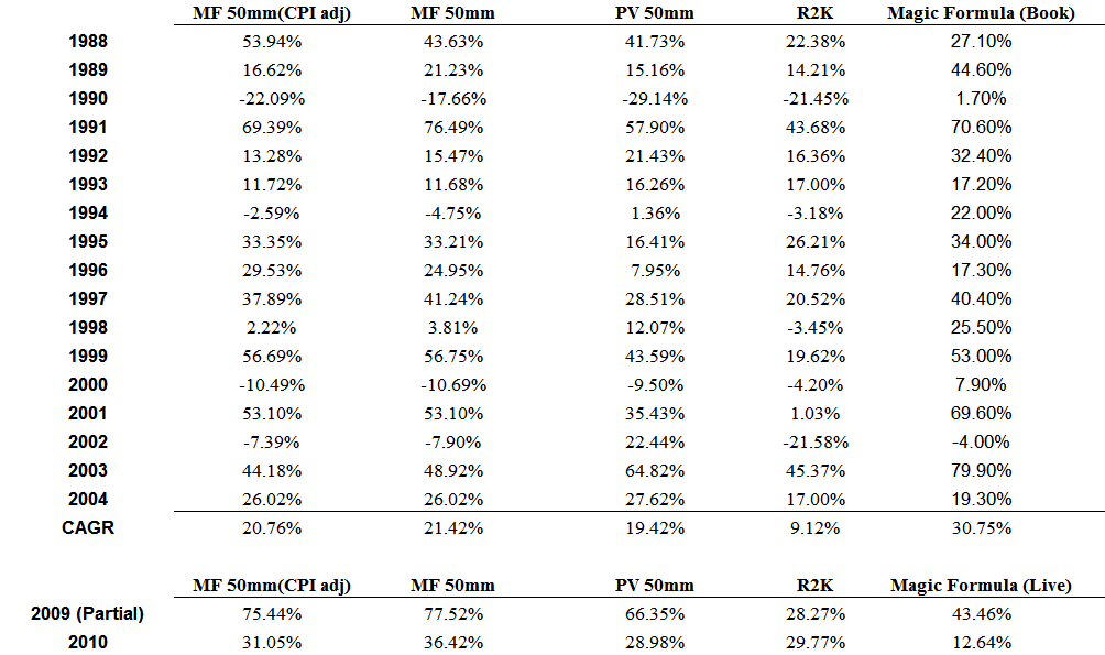
From a statistical standpoint, the MF 50mm (CPI adjusted), MF 50mm, and Profit and Value 50mm are a statistical tie–all have great returns over the limited time sample.

And while the MF returns are definitely higher when you allow for smaller stocks, the results still do not earn anywhere near 31% CAGR.

Some closer observations of our results versus the results from the book:

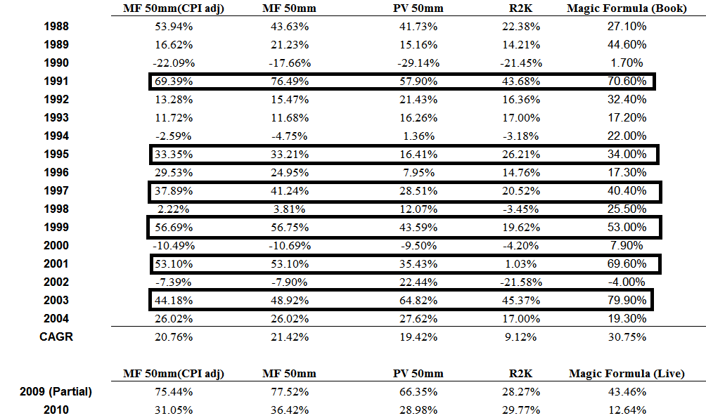
• For major “up” years, it seems that our backtest of the magic formula are very similar (especially from a statistical standpoint where the portfolios only have 30 names): 1991, 1995, 1997, 1999, 2001, and 2003.

 
• For “normal” up years, our backtest results essentially net out to be about the same.upon the original accrual anomaly?
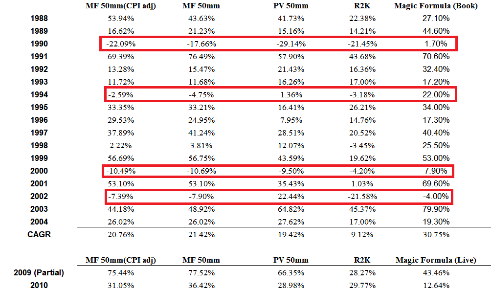
• The BIG difference is during down years: 1990, 1994, 2000, and 2002. For some reason, our backtest shows results which are roughly in line with the R2K (Russell 2000), but the MF results from the book present compelling upside returns during market downturns–so somehow the book results have negative beta during market blowouts? Weird to say the least…

We’d love to hear from someone else out there with the capability to do robust backtesting–perhaps the magic can be explained.

Some potential explanations:

1. My guess is the limited-size portfolio may be the answer to the discrepancy–a 1, 2, or 3 stock difference can have insane effects–hence the reason why decile or quantile portfolio performance (with a minimum of 100+ stocks)  is much more robust and credible.
2. Another option is that delistings were not appropriately accounted for in the book’s results (this might also explain why returns look great during market blowups…the exact time when delistings likely have largest effect on results). Richard Price has an excellent paper on the subject of delistings and highlights how important it is to properly deal with delistings data when backtesting “anomalies.”

The abstract from Professor Price’s paper:

“We show that tests of market effciency are sensitive to the inclusion of delisting firm-years. When included, trading strategy returns based on anomaly variables can increase (for strategies based on earnings, cash flows and the book-to-market ratio) or decrease (for a strategy based on accruals). This is due to the disproportionate number of delisting firm- years in the lowest decile of these variables. Delisting firm-years are most often excluded because the researcher does not correctly incorporate delisting returns, because delisting return data are missing or because other research design choices implicitly exclude them.”

Haugen’s Magic?

For sh$%s and giggles, I analysed the returns from Bob Haugen’s website. If you don’t know about Bob Haugen, then you don’t know about the original master of “quantitative value.” To put it simply, Bob took every factor in the book, ran a huge regression, and backed out all the variables that work the best. His factor model is the “Ferrari” of factor models.

How do Haugen’s returns  stack up to the MF and PV? (the returns are available starting in 1994 from his website).

We are looking at a small sample period, but wow–Haugen’s massive factor model looks to be the real magic.  Or course, the formula’s 126.13% return during 2003’s “Biblical scale small-cap move” certainly doesn’t hurt any of the strategies.

When we have some time (a lot of time!) we’ll re-backtest his strategy and see how it looks.

Enjoy the weekend.